Also available as: PDF.
See also: Experiment.
Approaches to Interpreter Composition
Abstract
In this paper, we compose six different Python and Prolog VMs into 4 pairwise compositions: one using C interpreters; one running on the JVM; one using meta-tracing interpreters; and one using a C interpreter and a meta-tracing interpreter. We show that programs that cross the language barrier frequently execute faster in a meta-tracing composition, and that meta-tracing imposes a significantly lower overhead on composed programs relative to mono-language programs.
1. Overview
Programming language composition aims to allow the mixing of programming languages in a fine-grained manner. This vision brings many challenging problems, from the interaction of language semantics to performance. In this paper, we investigate the runtime performance of composed programs in high-level languages. We start from the assumption that execution of such programs is most likely to be through composing language implementations that use interpreters and VMs, rather than traditional compilers. This raises the question: how do different styles of composition affect performance? Clearly, such a question cannot have a single answer but, to the best of our knowledge, this issue has not been explored in the past.
This paper’s hypothesis is that meta-tracing – a relatively new technique used to produce JIT (Just-In-Time) compilers from interpreters [8] – will lead to faster interpreter composition than traditional approaches. To test this hypothesis, we present a Python and Prolog composition which allows Python programs to embed and call Prolog programs. We then implement the composition in four different ways, comparing the absolute times and the relative cross-language costs of each. In addition to the ‘traditional’ approaches to composing interpreters (in C and upon the JVM), we also investigate the application of meta-tracing to interpreter composition. The experiments we then carry out confirm our initial hypothesis.
There is a long tradition of composing Prolog with other languages (with e.g. Icon [33], Lisp [36], and Smalltalk [21]) because one can express certain types of programs far easier in Prolog than in other languages. We have two additional reasons for choosing this pairing. First, these languages represent very different points in the language design space: Prolog’s inherently backtracking nature, for example, leads to a much different execution model than that of Python. It is therefore reasonable to assume that it is harder to optimise the composition of such languages than it would be if they were substantially similar. Second, each language has incarnations in several different language implementation paradigms, making our experiment practical. Few other languages meet both these criteria at the current time.
The four compositions we implemented are as follows: CPython-SWI composes two C interpreters; PyPy-SWI composes RPython and C interpreters; Unipycation composes two RPython interpreters; and Jython-tuProlog two JVM interpreters. CPython-SWI, PyPy-SWI, and Jython-tuProlog represent ‘traditional’ techniques to language composition; Unipycation embodies a new technique. Each composition implements exactly the same user-visible language, so composed programs run without change on each of the composed VMs. We have implemented the Python to Prolog interface as a mixture of pure Python code and code written in the language of the underlying system (RPython, C, Java), deliberately modelling how such libraries are typically implemented. Unipycation is an extension of work presented in a previous workshop paper [2], which we have since enhanced to allow full cross-language inlining. Note however, that unlike our previous work, this paper restricts itself to Python code calling Prolog, and not vice versa (some of the composed VMs are fundamentally unable to support the latter).
To address our hypothesis, we present a series of microbenchmarks, each designed to focus on a single aspect of cross-language performance, as well as a small set of (relatively) larger benchmarks which cross language barriers more freely. Each benchmark has both mono-language variants written in either Python or Prolog, and composed variants written in a mixture of Python and Prolog. We report our benchmark timings in absolute seconds, but also as ratios of the mono-language variants and Unipycation. The latter results allow us to understand the cost of moving from mono-language to composed variants, as well as the performance consequences of using meta-tracing for composed VMs. To ensure that our results are as robust as possible, we use the rigorous methodology of Kalibera/Jones; since we are, as far as we know, the first ‘users’ of this methodology, we also describe our experiences of it.
Our results break down as follows. First, as an unsurprising base-line, benchmarks which rarely cross the language barrier are dominated by the performance characteristics of the individual language implementations; put another way, the particular composition technique used makes little difference. Second, for those benchmarks which cross the language barrier frequently, Unipycation is, on average, significantly faster than PyPy-SWI; CPython-SWI is somewhat slower again; and Jython-tuProlog is hugely (unusably) slower. Third, Unipycation executes composed microbenchmarks in the same performance ballpark as the mono-language variants (at worst, well within an order of magnitude difference; and often only a few percent slower). By contrast, the next best performing composed VM PyPy-SWI is often at least 1–3 orders of magnitude worse than the mono-language variants. Bearing in mind the dangers of generalising from any specific set of benchmarks, we consider these results to validate the paper’s hypothesis.
Our contributions are as follows:
- We present a viable Python/Prolog composition and show four different implementations each using a different composition style.
- We present the first experiment designed to help understand the effects of different composition styles upon performance.
- We thoroughly analyse and discuss the results of the experiment, breaking down the impact that each composition style has on performance.
The experiments contained in this paper are downloadable and repeatable from:
This paper is structured as follows. We briefly introduce meta-tracing (Section 2) and Prolog for those readers who may be unfamiliar, or rusty, with either. After introducing the generic Unipycation interface, including an example Python and Prolog composition with an implementation of Connect 4 (Section 4.2), we then describe the four implementations of this interface (Section 5). The experimental setup (Section 6) is followed by a quantitative analysis of its results (Section 7) and a qualitative discussion (Section 8).
2. Meta-tracing
This section briefly introduces the concept of meta-tracing. Meta-tracing takes as input an interpreter, and from it creates a VM containing both the interpreter and a tracing JIT compiler [34, 38, 6, 44, 4]. Although tracing is not a new idea (see [1, 17]), it traditionally required manually implementing both interpreter and trace compiler. Meta-tracing, in contrast, automatically generates a trace compiler from an interpreter. At run-time, user programs running in the VM begin their execution in the interpreter. When a ‘hot loop’ in the user program is encountered, the actions of the interpreter are traced (i.e. recorded), optimised, and converted to machine code. Subsequent executions of the loop then use the fast machine code version rather than the slow interpreter. Guards are left behind in the machine code so that execution can revert back to the interpreter when the path recorded by the trace differs from that required.
Meta-tracing works because of the particular nature of interpreters. Irrespective of whether they operate on bytecode or ASTs, are iterative or recursive, interpreters are fundamentally a large loop: ‘load the next instruction; perform the associated actions; repeat the loop’. To generate a tracing JIT, the language implementer annotates the interpreter to inform the meta-tracing system when a loop1 at position pc (program counter) has been encountered; the meta-tracing system then decides if the loop has been encountered often enough to start tracing. The annotation also tells the meta-tracing system that execution of the program at position pc is about to begin and that if a machine code version is available, it should be used; if not, the standard interpreter will be used.
The main extant meta-tracing language is RPython, a statically-typed subset of Python which translates to C. RPython’s type system is similar to Java’s, extended with further analysis, e.g. to ensure that list indices are not negative. Users can influence the analysis with assert statements, but otherwise it is fully automatic. Unlike seemingly similar languages (e.g. Slang [25] or PreScheme [32]), RPython is more than just a thin layer over C: it is, for example, fully garbage collected and has several high-level datatypes (e.g. lists and dictionaries). Despite this, VMs written in RPython have performance levels which far exceed traditional interpreter-only implementations [8].
Meta-tracing is appealing for composed VMs because it holds the prospect of achieving meaningful cross-language optimisations for little or no effort. We explore this in the context of Unipycation in Section 5.3.
3. Prolog Background
While we assume that most readers have a working knowledge of a mainstream imperative language such that they can understand Python, we can not reasonably make the same assumption about Prolog. This section serves as a brief introduction to Prolog for unfamiliar readers (see e.g. [9] for more details). Those familiar with Prolog will notice a distinct imperative flavour to our explanations. This is intentional, given the paper’s likely audience, but nothing we write should be considered as precluding the logic-based view of Prolog.
Prolog is a rule-based logic programming language whose programs consist of a database of predicates which is then queried. A predicate is related to, but subtly different from, the traditional programming language concept of a function. Predicates can be loosely thought of as overloaded pattern-matching functions that can generate a stream of solutions (including no solutions at all). Given a database, a user can then query it to ascertain the truth of an expression.
Prolog supports the following data types:
- Numeric constants: Integers and floats.
- Atoms: Identifiers starting with a lowercase letter e.g. chair.
- Terms: Composite structures beginning with a lowercase letter e.g. vector(1.4, 9.0). The name (e.g. vector) is the term’s functor, the items within parentheses its arguments.
- Variables: Identifiers beginning with either an uppercase letter (e.g. Person) or an underscore. A variable denotes an as yet unknown value that may become known later when a concrete value is bound to the variable.
- Lists: Lists are made out of cons cells, which are simply terms of the functor ’.’. Since lists are common, and the ’.’ syntax rather verbose, lists can be expressed using a comma separated sequence of elements enclosed inside square brackets. For example, the list [1,2,3] is equivalent to ’.’(1, ’.’(2, ’.’(3, []))). Furthermore, a list can be denoted in terms of its head and tail, for example [1 | [2, 3]] is equivalent to [1,2,3].
To demonstrate some of these concepts, consider the Prolog rule database shown in Listing 1. The edge predicate describes a directed graph which may, for example, represent a transit system such as the London Underground. The path predicate accepts four arguments and describes valid paths of length MaxLen or under, from the node From to the node To, as the list Nodes. In this example, a, b, …, g are atoms. The expression edge(a, c) defines a predicate called edge which is true when the atoms a then c are passed as arguments. The expression path(From, To, MaxLen, Nodes, 1) is a call to the path predicate passing as arguments, four variables and a integer constant.
1edge(a, c). edge(c, b). edge(c, d). edge(d, e).
2edge(b, e). edge(c, f). edge(f, g). edge(e, g).
3edge(g, b).
4
5path(From, To, MaxLen, Nodes) :-
6 path(From, To, MaxLen, Nodes, 1).
7
8path(Node, Node, _MaxLen, [Node], _Len).
9path(From, To, MaxLen, [From | Ahead ], Len) :-
10 Len < MaxLen, edge(From, Next),
11 Len1 is Len + 1,
12 path(Next, To, MaxLen, Ahead, Len1).
Queries can either succeed or fail. For example, running the query edge(c, b) (“is it possible to transition from node c to node b?”) against the above database succeeds, but edge(e, f) (“is it possible to transition from node e to node f?”) fails. When a query contains a variable, Prolog searches for solutions, binding values to variables. For example, the query edge(f, Node) (“which node can I transition to from f?”) binds Node to the atom g. Queries can produce multiple solutions. For example, path(a, g, 7, Nodes) (“Give me paths from a to g of maximum length 7”) finds several bindings for Nodes: [a, c, b, e, g], [a, c, d, e, g], [a, c, f, g], and [a, c, f, g, b, e, g].
Solutions are enumerated by recording choice points where more than one rule is applicable. If a user requests another solution, or if an evaluation path fails, Prolog backtracks and explores alternative search paths by taking different decisions at choice points. In the above example, edge(From, Next) (line 10) can introduce a choice point, as there can be several ways of transitioning from one node to the next.
4. The Unipycation interface
Unipycation is both an implementation of a Python and Prolog composition, and an interface which other implementations can target. In this paper we provide 4 composed VMs which, while they differ significantly internally, presents the same interface to the programmer. All Unipycation programs start with Python code, subsequently using the uni module to gain access to the Prolog interpreter, as in the following Unipycation program:
1import uni
2e = uni.Engine("""
3 % parent(ParentName, ChildName, ChildGender)
4 parent(jim, lucy, f). parent(evan, lily, f).
5 parent(jim, sara, f). parent(evan, emma, f).
6 parent(evan, kyle, m).
7
8 siblings(Person1, Person2, Gender) :-
9 parent(Parent, Person1, Gender),
10 parent(Parent, Person2, Gender),
11 Person1 \= Person2.
12""")
13
14for (p1, p2) in e.db.siblings.iter(None, None, "f"):
15 print "%s and %s are sisters" % (p1, p2)
The Python code first imports the uni module and creates an instance of a Prolog engine (line 2). In this case, the engine’s database is passed as a Python string (lines 3-11 inclusive), although databases can be loaded by other means (e.g. from a file). The Prolog database models a family tree with a series of parent facts. The siblings predicate can then be used to infer pairs of same-sex siblings. This example queries the Prolog database for all pairs of sisters (line 14) and successively prints them out (line 15). The Prolog database is accessed through the db attribute of the engine (e.g. e.db.siblings). Calling a Prolog predicate as if it were a Python method transfers execution to Prolog and returns the first solution; if no solution is found then None is returned. Predicates also have an iter method which behaves as a Python iterator, successively generating all solutions (as shown in the example on line 14). Solutions returned by the iterator interface are generated in a lazy on-demand fashion.
Calling to, and returning from, Prolog requires datatype conversions. Python numbers map to their Prolog equivalents; Python strings map to Prolog atoms; and Python (array-based) lists map to Prolog (cons cell) lists. A Python None is used to represent a (distinct) unbound variable. Composite terms (not shown in the example) are passed as instances of a special Python type uni.Term, instantiated by a call to a method of the engine’s terms attribute. For example, a term equivalent to vec(4, 6) is instantiated by executing e.terms.vec(4, 6). Prolog solutions are returned to Python as a tuple, with one element for each None argument passed.
When run, Listing 2 generates the following output:
4.1. High-Level and Low-Level Interface
Although it may not be evident from studying Unipycation code, our composed VMs are implemented in two distinct levels. The uni module (shown in the previous section) exposes a high-level programming interface written in pure Python. This allows us to use it unchanged across our four composed VMs. At a lower-level, each of the compositions exposes a fixed API for the uni module to interface with. This split has several advantages: it maximises code sharing between the compositions; makes it easier to experiment with different uni interface designs; and models a typical approach used by many Python libraries that wrap non-Python code such as C libraries.
The low-level interface provides a means to create a Prolog engine with a database. It also provides an iterator-style query interface and some basic type conversions—higher-level conversions are delegated to the uni module. In particular, Prolog terms have the thinnest possible wrapper put around them. When returning solutions to Python, the high-level interface must perform a deep copy on terms, as most of the Prolog implementations garbage collect, or modify, them when a query is pumped for more solutions.
The low-level interface is an implementation detail that is not intended for end-users. Failing to follow certain restrictions leads to undesirable behaviour, from returning arbitrary results to segmentation faults (depending on the composed VM). The uni module follows these restrictions by design.
4.2. An Example
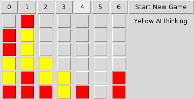
To show what sorts of programs one might wish to write with the Unipycation interface, we present a small case study of a Connect 4 implementation. Connect 4 is a well known strategy game, first released in 1974. The game involves two players (red and yellow), and a vertically standing grid-like board, divided into 6 rows and 7 columns. Players take turns dropping one of their coloured counters into a column. The first player to place 4 counters in a contiguous horizontal, vertical, or diagonal line wins.
Connect 4 has two distinct aspects: a user interface and an AI player. Without wishing to start a war between fans of either language, we humbly suggest that Python is better suited to expressing the GUI, whereas Prolog is better suited to expressing the behaviour of an AI player. Our implementation follows this pattern, and has a Python GUI of 183LoC and a Prolog AI player of 168LoC.
The basic operation of the case study is as follows. The Python part of the program performs all interactions with users and stores the state of the board. After every move, the Python part divides the state of the board into two lists (reds and yellows), encoding counter positions as Prolog terms (e.g. a counter at row one, column two is encoded as c(2, 1)). Unipycation’s Python → Prolog interface is then used to query the Prolog has_won predicate passing as arguments the two lists and a final unbound variable. If the Prolog interpreter finds a binding to the variable, then the game has finished, and the last player to move has won.
If no player has won, and the next player to move is the AI opponent, the Python part hands over to the Prolog AI player. To decide a good move, the computer opponent uses a bounded-depth minimax solver [41, 42] implemented efficiently using alpha-beta pruning [15]; we used Bratko’s alpha-beta framework as a reference implementation [9, p. 586]. This approach considers the game as a tree of potential moves, where each move is characterised by the positions of the counters (again as two lists) and whose move it is next. Each move has an associated cost which is used as a basis for deciding a good move. We model Connect 4 as a zero sum game, so for one player a good move minimises the cost, whereas for the other player a good move maximises the cost. The alpha-beta framework requires us to define three predicates: one to tell the framework whose turn it is in a given position, one to calculate all possible next moves, and one to calculate the cost of a move. Given these predicates, the alpha-beta framework can make an informed decision about the best move for the computer opponent. Once the best move has been chosen, it is passed back to Python and the game state is updated to reflect the AI player’s move.
We discuss our experiences of using Unipycation for the case study in Section 8.
5. The Composed VMs
In this section we describe our four composed VMs. Each takes two existing language implementations – one Python, and one Prolog – and glues them together. The language implementations and the versions used, are shown in Table 1; the size of the glue is shown in Table 2. To ensure our experiment is repeatable, we used only open source language implementations.
| Implementation | Version |
| CPython | 2.7.6 |
| Jython | HG aa042b69bdda |
| SWI Prolog | 6.6.1 |
| PyPy | HG fa985109fcb9 |
| Pyrolog | HG cab0c5802fe9 |
| tuProlog | SVN 1263 |
| VM | LoC |
| CPython-SWI | 800 (Python) |
| PyPy-SWI | See CPython-SWI (same code) |
| Unipycation | 650 (RPython) |
| Jython-tuProlog | 350 (Python) |
5.1. CPython-SWI
CPython-SWI composes two interpreters written in C: CPython and SWI Prolog [43]. CPython is the de-facto standard implementation of Python and SWI Prolog is the most popular open-source Prolog interpreter.
CPython-SWI’s glue code is the largest of the composed VMs. This reflects the intricacies of mixing together low-level interpreters with different garbage collectors (etc.). To make our life somewhat easier, the glue code was written in Python using the CFFI library.2 On first import, CFFI emits C code which is compiled into a CPython extension and loaded; the extension in turn loads SWI Prolog as a dynamic library, meaning, in essence, that the composition occurs at the C level. Around 430LoC relate to CFFI from which around 2KLoC of C code are generated. To give a flavour of our implementation style, Listing 3 shows an excerpt from the CPython-SWI conversion code (conversion code for the other VMs looks much the same). Implementing CPython-SWI required no modifications to either CPython or SWI Prolog.
1def py_of_pro(pro_term):
2 lib = C._libpl
3 pl_type = lib.PL_term_type(pro_term)
4 if pl_type == lib.PL_ATOM:
5 return py_str_of_pro_atom(pro_term)
6 elif pl_type == lib.PL_TERM:
7 return py_term_of_pro_term(pro_term)
8 elif pl_type == ...:
9 ...
10
11def py_str_of_pro_atom(pro_atom):
12 return C.get_str(pro_atom)
13
14def py_term_of_pro_term(pro_term):
15 return CoreTerm.from_pl_term(pro_term)
5.2. PyPy-SWI
PyPy-SWI is a simple variant of CPython-SWI, swapping CPython for PyPy. Because we used CFFI for CPython-SWI’s glue code, ‘creating’ PyPy-SWI is simply a matter of invoking the same (unchanged) code under PyPy. PyPy-SWI is interesting in that it composes a JITing VM (PyPy) with a traditional interpreter (SWI Prolog).
5.3. Unipycation
Unipycation composes two RPython (see Section 2) interpreters: PyPy [35] and Pyrolog [7]. PyPy is a fast [8], industrial strength implementation of Python 2.7.3 and has been widely adopted in the open-source community. Pyrolog has its origins in a research project investigating the application of meta-tracing to logic programming. As PyPy modules need to be statically compiled into the VM, the low-level interface required adding a module to PyPy’s source. Pyrolog is, from this paper’s perspective, unmodified.3 In the rest of this subsection, we explain how meta-tracing enables cross-language optimisations, and how Unipycation can inline Prolog code called from Python.
Each of Unipycation’s constituent interpreters has its own meta-tracing JIT, such that running Python or Prolog code under Unipycation is as fast as running it in a stand-alone PyPy or Pyrolog VM. Most of Unipycation’s optimisations are inherent to meta-tracing. Both PyPy and Pyrolog are optimised for meta-tracing in the sense that their implementation has, where necessary, been structured according to meta-tracing’s demands. Such structuring is relatively minor (see [8] for more details): most commonly, tracing annotations are added to the interpreter to provide hints to the tracer (e.g. “this RPython function’s loops can safely be unrolled”). Less commonly, code is e.g. moved into its own function to allow an annotation to be applied. To improve the performance of Unipycation, we added ten such annotations, but PyPy and Pyrolog themselves were mostly left unchanged. This is not to suggest that the two interpreters have identical execution models: PyPy is a naive recursive bytecode interpreter, whereas Pyrolog uses continuation-passing style (in fact, Pyrolog uses two continuations: one for success and one for failure [7] using a trampoline).
A tracing JIT’s natural tendency to aggressively type-specialise code (see [16]) is important in reducing the overhead of object conversions between interpreters. Tracing a call from one language to the other naturally traces the object conversion code in the uni module, type specialising it. In essence, Unipycation assumes that the types of objects converted at a given point in the code will stay relatively constant; similar assumptions are the basis of all dynamically typed language JITs. Type specialisation leaves behind a type guard, so that if the assumption of type constancy is later invalidated, execution returns to the interpreter. If, as is likely, the object conversion is part of a bigger trace with a previous equivalent type guard, RPython’s tracing optimiser will remove the redundant type guard from the object conversion.
A related optimisation occurs on the wrapped objects that are created by cross-interpreter object conversion. The frequent passing of objects between the two interpreters would seem to be inefficient, as most will create a new wrapper object each time they are passed to the other interpreter. Most such objects exist only within a single trace and their allocation costs are removed by RPython’s escape analysis [5].
The final optimisation we hope to inherit from meta-tracing is inlining. While it is relatively easy to inline Python code called from Prolog, the other way around – which is of rather more importance to this paper – is complicated by tracing pragmatics. In essence, the tracer refuses to inline functions which contain loops, since it is normally better to trace them separately. Languages like Python can trivially detect most loops statically (e.g. the use of a while loop in a function). Prolog loops, in contrast, are tail-recursive calls, which, due to Prolog’s highly dynamic nature, can often only be detected reliably at run-time. By default, the tracer therefore considers every call to Prolog as a potential loop and does not inline any of them.
Our solution is simple, pragmatic, and can easily be applied to similar languages. Rather than trying to devise complex heuristics for determining loops in Prolog, we always inline a fixed number of Prolog reduction steps into Python. If the Prolog predicate finishes execution within that limit, then it is fully inlined. If it exceeds the limit, a call to the rest of the predicate is emitted, stopping inlining at that point. This means that if the Prolog predicate being inlined does contain a loop, then part of it is unrolled into the machine code for the outer Python function. Remaining loop iterations (if any) are executed via an explicitly inserted call to the rest of the predicate. This approach allows small predicates to benefit from inlining, while preventing large predicates from causing unpalatable slow-downs. Ultimately the effect is similar to the meta-tracer’s normal inlining behaviour in mono-language implementations like PyPy.
5.4. Jython-tuProlog
Jython-tuProlog composes two languages atop the JVM: Jython4 and tuProlog [13]. Jython is the only mature Python JVM implementation and targets Python 2.7. We chose tuProlog since it is the most complete embeddable JVM Prolog implementation we know of.5 Neither Jython nor tuProlog were altered in realising Jython-tuProlog.
6. Experimental Setup
This paper’s main hypothesis is as follows:
- H1 Meta-tracing leads to faster interpreter composition than traditional approaches.
To address this hypothesis, we run a number of benchmarks across the four compositions we created. The benchmarks are organised into two groups: microbenchmarks, which aim to test a single aspect of cross-language composition; and larger benchmarks, which aim to test several aspects at once.
Running such benchmarks in a fair, consistent manner is tricky: bias – often unintentional and unnoted – is rife. This is particularly true for virtual machines with complex JIT compilers and garbage collectors. These components bring in many sources of non-determinism, many of them related to code and data layout differences in the JIT-compiled code, which can lead to significant performance effects via different caching behaviour [20, 18]. The fact that we combine VMs that each have their individual effects exacerbates the issue.
We therefore base our experimental methodology on the statistically rigorous Kalibera/Jones method [30]. Since, to the best of our knowledge, we are the first people apart from Kalibera/Jones to do so, we assume that most of our readers are unfamiliar with this method, and give a gentle introduction in Section 6.3.
6.1. Microbenchmarks
We have designed six microbenchmarks that measure the costs of specific activities when crossing language boundaries. Each benchmark consists of a ‘caller’ function and ‘callee’ function:
- SmallFuncThe caller passes an integer to a tiny callee which returns the integer, incremented by 1.
- L1A0R Both the caller and the callee functions are loops. The callee receives a single integer argument.
- L1A1R Both the caller and callee are loops. The callee receives a single integer argument and returns a single integer result.
- NdL1A1R The caller invokes the callee in a loop. The callee produces more than one integer result (by returning an iterator in Python, and leaving a choice point in Prolog). The caller asks for all of the results (with a for loop in Python, and with a failure-driven loop in Prolog).
- Lists The callee produces a list, and the caller consumes it (e.g. iterates over all its elements). The lists are converted between Prolog linked lists and Python array-based lists when passing the language barrier.
- TCons The caller walks a linked list which is produced by the callee using Prolog terms.
Each of the microbenchmarks comes in three variants:
- Python Both caller and callee are Python code.
- Prolog Both caller and callee are Prolog code.
- Python → Prolog The caller is Python code, the callee is Prolog code.
The first two variants give us a baseline, while the latter measures cross-language calling. Whilst we have created Prolog → Python variants of the benchmarks, only Unipycation can execute them (see Section 8.2) so we do not consider them further.
6.2. Larger Benchmarks
The limitations of microbenchmarks are well known. Since there are no pre-existing Unipycation programs, we have thus created three (relatively) larger benchmarks, based on an educated guess about the style of programs that real users might write. While we would have liked to create a larger set of bigger benchmarks, we are somewhat constrained by inherent limitations in Jython-tuProlog and CPython-SWI, which accept a narrower range of programs than Unipycation itself. However, while we do not claim that these benchmarks are definitely representative of programs that other people may find Unipycation useful for, they do enable us to examine a different class of behaviours than the microbenchmarks.
Each of the benchmarks has two variants: Prolog only; and composed Python / Prolog. The composed benchmarks can be broadly split into two: those that cross the language barrier frequently (SAT model enumeration) and those that spend most of their time in Prolog (Connect 4 and the Tube benchmark).
6.2.1. Connect 4
This benchmark is based on the implementation described in Section 4.2. To make a sensible benchmark, we removed the GUI, made the AI player deterministic, and pitted the AI player against itself. We measure the time taken for a complete AI versus AI game to execute.
6.2.2. Tube Route Finder
Given a start and end station, this benchmark finds all the shortest possible routes6 through an undirected graph representing the London Underground.7 This is achieved by an iterative deepening depth-first search, monotonically increasing the depth until at least one solution is found; backtracking is used to enumerate all shortest routes. In the composed variant, Python increases the depth in a loop, with each iteration invoking Prolog to run a depth first search. Despite this, the composed benchmark intentionally spends nearly all of its time in Prolog and is thus a base-case of sorts for composed programs which do not cross the language barrier frequently. We measure the time taken to find routes between a predetermined pair of stations.
6.2.3. SAT Model Enumeration
This benchmark exhaustively enumerates the solutions (models) to propositional formulas using Howe and King’s small Prolog SAT solver [23]. As the models are enumerated, we count the number of propositional variables assigned to true. The composed variant uses Python for the outer model enumeration loop. We measure the time taken to count the true literals appearing in the models of a SAT instance borrowed from the SATLIB suite [22].
Note that since tuProlog does not support coroutines, this benchmark cannot be run under Jython-tuProlog.
6.3. Kalibera/Jones Method
Benchmarks often exhibit non-deterministic behaviour which goes unnoticed or unexplained, distorting results and our perceptions of them. In computing, the default response has mostly been to ignore the issue and hope for the best [40]. To help make our benchmarks as fair and representative as reasonably possible, we have adopted the more statistically rigorous Kalibera/Jones method [30]. The basic aim of the method is to determine a suitable number of experimental repetitions for the various levels involved in benchmarking, whilst retaining a reasonable level of precision. It also gives a mathematically sound method for computing relative speed-ups of benchmarks, including confidence intervals. We now give a brief overview of the method and detail how we applied it to our benchmarks.
The method first requires us to consider the levels involved in the experiment. At each of the levels there is an opportunity to repeat experimentation. Typical levels for a VM-based language (from low to high) might be: the iterations level, sequential repetitions within a process; the executions level, repetitions of the iteration level, each time spawning a fresh process; and the VMs level, repetitions of compiling the VM. Multiple levels need to be considered because benchmarks can be non-deterministic at one level, but not at another. For example, benchmarks which are non-deterministic in their initialisation code will exhibit variation at the executions level but not the iterations level. Cursory inspection showed that for our experiments there was no meaningful variation at the VM level, so we concentrated on the iterations and executions levels.
Having identified the appropriate levels, a dimensioning run of the experiment is performed with many repetitions to determine each benchmark’s variance at each level. The ordered measurements are first used to determine if each benchmark reaches an initialised state: the point at which subsequent runs are no longer subject to start-up costs (e.g. JIT warmup). This is determined by plotting a graph of sequential run times and manually determining when such a state has been reached. The method also gives a process to determine if a benchmark reaches an independent state. If the benchmark reaches the independent state, then we can be sure that the measurements taken for subsequent iterations level runs are in no way correlated with previous runs. This is a useful property since it means that one can safely take a sample of measurements at any point from the independent state onwards. Since some experiments may never converge upon the independent state, the methodology also provides a fallback method, whereby a single consistent post-initialised iteration (in our case, the first) is taken.
For dimensioning, we used 10 runs at the iterations level and 10 at the executions level – i.e. 10 ∗ 10 = 100 runs – which was large enough to give useful data in a somewhat reasonable time frame (about 3 weeks). To make our life easier, for each VM we took the maximum initialisation sequence position (rather than using a manually determined value for each VM / benchmark combination). We set the initialisation state as iteration #6 for all VMs except for CPython-SWI which, not using a JIT, reaches an initialised state at iteration #2. Since Jython-tuProlog is so much slower than other implementations, we were unable to do a full dimensioning run in reasonable time; we thus used a subset of the benchmarks to determine that it also reached the initialisation state at iteration #6.
Given data from a dimensioning run, one can then compute the amount of variance introduced at each level. To our surprise, the variation in our benchmarks was consistently much higher at the executions level than the iterations level. The method’s heuristic therefore suggested that, since there was little variation at the iterations level, we need only measure the time taken for a single post-initialisation iteration. Since the methodology does not give a method for choosing a number of repetitions for the highest level of experimentation, we chose 30 repetitions for the executions level. However, we were forced to lower this for Jython-tuProlog, which is rather slow (30 repetitions would lead to a running time of 3 months), instead using 10 repetitions for Jython-tuProlog’s execution level.
With the repetition counts determined, we then ran the real experiment and computed 99% confidence intervals. As suggested by Kalibera/Jones, we used the bootstrap re-sampling method with 10000 iterations to compute the confidence intervals, which has the advantage that we are not required to make any assumptions about the shape of the underlying distribution.
Our experiments were run on an otherwise idle system with a 4GHz Intel Core i7-4790K CPU (with turbo mode disabled), 24 GiB RAM, and running Debian Linux 7.7 in 64 bit mode. All timings are wall-clock with a sub-microsecond resolution.
6.4. Investigating conversion and the effect of meta-tracing
In addition to measuring the raw benchmarks, we perform two additional experiments designed to help us address two additional hypotheses:
- H2 Cross-language inlining is a significant part of meta-tracing’s benefits.
- H3 Meta-tracing reduces data conversion costs.
To test hypothesis H2, we created a variant of Unipycation that completely disables inlining across the Python/Prolog boundary and ran all benchmarks on that variant.
To test hypothesis H3, we created another benchmark variant Python →nc Prolog which measures how fast the benchmarks run with zero-cost conversions. For each benchmark we hand-crafted two versions: one that computes and records the arguments and results for every cross-interpreter call; and one that uses the precomputed arguments and results. The latter variant is the one for which we measure times.
7. Experimental Results
Tables 3, 4, and 6 show the raw results from running the benchmarks against the four composed VMs. Table 3 shows how often each benchmark crosses the language barrier and how many objects are converted in those crossings; Tables 4 and 6 show benchmark timings in absolute seconds.
Tables 5 and 7 show two subtly different things. First, the relative costs of moving from a mono-language to a composed VM; informally, we say the composed VM is efficient if the relative cost of the composed variant is ‘close’ to the mono-language variant. Second, the slow-down of using a composed VM relative to Unipycation.
In the rest of this section, we analyse these results in detail and share our insights
into them.
| Benchmark | Crossings | Objs converted |
| SmallFunc | 1000000 | 5000000 |
| L1A0R | 100000 | 100000 |
| L1A1R | 100000 | 300000 |
| NdL1A1R | 100300000 | 100300000 |
| TCons | 100000 | 400400000 |
| Lists | 100000 | 100500000 |
| sat-models | 41505 | 12579962 |
| tube | 558 | 3984 |
| connect4 | 126 | 14889 |
| VM | Benchmark | Python | Prolog | Python → Prolog
| |||
|
CPython-SWI | SmallFunc | 0.933s | ±0.002 | 1.983s | ±0.011 | 196.000s | ±4.225 |
| L1A0R | 3.150s | ±0.008 | 5.712s | ±0.035 | 6.895s | ±0.024 | |
| L1A1R | 4.820s | ±0.006 | 15.279s | ±0.054 | 16.378s | ±0.056 | |
| NdL1A1R | 6.637s | ±0.011 | 12.186s | ±0.129 | 427.917s | ±3.239 | |
| TCons | 237.952s | ±1.209 | 36.034s | ±0.100 | 1451.516s | ±7.143 | |
| Lists | 9.328s | ±0.009 | 19.463s | ±0.060 | 1379.922s | ±7.618 | |
|
PyPy-SWI | SmallFunc | 0.006s | ±0.001 | 1.986s | ±0.014 | 20.840s | ±0.403 |
| L1A0R | 0.049s | ±0.002 | 5.714s | ±0.042 | 5.774s | ±0.019 | |
| L1A1R | 0.074s | ±0.003 | 15.232s | ±0.039 | 14.628s | ±0.048 | |
| NdL1A1R | 0.423s | ±0.010 | 12.171s | ±0.119 | 50.424s | ±0.529 | |
| TCons | 5.576s | ±0.032 | 36.040s | ±0.057 | 104.392s | ±1.284 | |
| Lists | 0.701s | ±0.003 | 19.472s | ±0.088 | 71.818s | ±0.341 | |
|
Unipycation | SmallFunc | 0.008s | ±0.000 | 0.048s | ±0.007 | 0.010s | ±0.001 |
| L1A0R | 0.045s | ±0.002 | 0.047s | ±0.003 | 0.045s | ±0.001 | |
| L1A1R | 0.069s | ±0.003 | 0.071s | ±0.003 | 0.074s | ±0.003 | |
| NdL1A1R | 0.422s | ±0.000 | 0.442s | ±0.016 | 2.493s | ±0.019 | |
| TCons | 4.754s | ±0.035 | 2.143s | ±0.003 | 28.871s | ±0.449 | |
| Lists | 0.700s | ±0.002 | 1.252s | ±0.002 | 4.176s | ±0.012 | |
|
Jython-tuProlog | SmallFunc | 0.700s | ±0.013 | 23.788s | ±0.080 | 313.299s | ±3.294 |
| L1A0R | 1.104s | ±0.007 | 153.766s | ±1.685 | 150.828s | ±1.032 | |
| L1A1R | 1.707s | ±0.062 | 222.879s | ±0.620 | 220.224s | ±1.994 | |
| NdL1A1R | 5.524s | ±0.134 | 1880.981s | ±7.642 | 2000.043s | ±15.500 | |
| TCons | 544.376s | ±6.075 | 7845.380s | ±28.407 | 8001.564s | ±26.390 | |
| Lists | 5.114s | ±0.079 | 7043.844s | ±15.929 | 5266.634s | ±13.188 | |
| VM | Benchmark | Python→Prolog Python | Python→Prolog Prolog | Python→Prolog
Unipycation | |||
|
CPython-SWI | SmallFunc | 210.060× | ±4.465 | 98.840× | ±2.188 | 20433.776× | ±1381.309 |
| L1A0R | 2.189× | ±0.009 | 1.207× | ±0.009 | 151.951× | ±3.853 | |
| L1A1R | 3.398× | ±0.012 | 1.072× | ±0.005 | 222.353× | ±10.662 | |
| NdL1A1R | 64.473× | ±0.493 | 35.114× | ±0.452 | 171.661× | ±1.860 | |
| TCons | 6.100× | ±0.044 | 40.281× | ±0.232 | 50.276× | ±0.811 | |
| Lists | 147.939× | ±0.842 | 70.901× | ±0.454 | 330.461× | ±2.112 | |
|
PyPy-SWI | SmallFunc | 3759.944× | ±535.177 | 10.494× | ±0.219 | 2172.673× | ±150.436 |
| L1A0R | 118.906× | ±5.622 | 1.010× | ±0.008 | 127.247× | ±3.153 | |
| L1A1R | 197.594× | ±8.467 | 0.960× | ±0.004 | 198.598× | ±9.384 | |
| NdL1A1R | 119.137× | ±2.999 | 4.143× | ±0.062 | 20.228× | ±0.263 | |
| TCons | 18.721× | ±0.251 | 2.897× | ±0.035 | 3.616× | ±0.072 | |
| Lists | 102.497× | ±0.646 | 3.688× | ±0.025 | 17.199× | ±0.096 | |
|
Unipycation | SmallFunc | 1.276× | ±0.081 | 0.201× | ±0.038 | 1.000× | |
| L1A0R | 1.005× | ±0.053 | 0.957× | ±0.057 | 1.000× | ||
| L1A1R | 1.072× | ±0.071 | 1.034× | ±0.069 | 1.000× | ||
| NdL1A1R | 5.902× | ±0.044 | 5.635× | ±0.216 | 1.000× | ||
| TCons | 6.073× | ±0.106 | 13.471× | ±0.208 | 1.000× | ||
| Lists | 5.969× | ±0.025 | 3.335× | ±0.010 | 1.000× | ||
|
Jython-tuProlog | SmallFunc | 447.378× | ±9.737 | 13.170× | ±0.146 | 32662.702× | ±2186.768 |
| L1A0R | 136.595× | ±1.257 | 0.981× | ±0.013 | 3324.147× | ±87.511 | |
| L1A1R | 128.989× | ±5.334 | 0.988× | ±0.009 | 2989.890× | ±140.681 | |
| NdL1A1R | 362.045× | ±9.169 | 1.063× | ±0.009 | 802.325× | ±8.918 | |
| TCons | 14.699× | ±0.178 | 1.020× | ±0.005 | 277.151× | ±4.256 | |
| Lists | 1029.866× | ±15.745 | 0.748× | ±0.003 | 1261.242× | ±4.698 | |
Python
| VM | Benchmark | Prolog | Python → Prolog
| ||
|
CPython-SWI | sat-models | 3.779s | ±0.090 | 91.205s | ±0.629 |
| tube | 0.272s | ±0.001 | 0.286s | ±0.001 | |
| connect4 | 14.172s | ±0.033 | 14.324s | ±0.036 | |
|
PyPy-SWI | sat-models | 3.148s | ±0.006 | 12.156s | ±0.208 |
| tube | 0.263s | ±0.002 | 0.265s | ±0.001 | |
| connect4 | 14.172s | ±0.035 | 14.243s | ±0.045 | |
|
Unipycation | sat-models | 1.958s | ±0.024 | 2.862s | ±0.021 |
| tube | 2.348s | ±0.026 | 2.381s | ±0.036 | |
| connect4 | 7.533s | ±0.047 | 10.783s | ±0.078 | |
|
Jython-tuProlog | sat-models | n/a | n/a | ||
| tube | 435.555s | ±1.644 | 411.496s | ±0.607 | |
| connect4 | 278.352s | ±0.787 | 268.351s | ±1.606 | |
| VM | Benchmark | Python→Prolog Prolog | Python→Prolog
Unipycation | ||
|
CPython-SWI | sat-models | 24.137× | ±0.599 | 31.871× | ±0.310 |
| tube | 1.052× | ±0.005 | 0.120× | ±0.002 | |
| connect4 | 1.011× | ±0.004 | 1.328× | ±0.010 | |
|
PyPy-SWI | sat-models | 3.862× | ±0.065 | 4.248× | ±0.076 |
| tube | 1.008× | ±0.009 | 0.111× | ±0.002 | |
| connect4 | 1.005× | ±0.004 | 1.321× | ±0.010 | |
|
Unipycation | sat-models | 1.462× | ±0.021 | 1.000× | |
| tube | 1.014× | ±0.019 | 1.000× | ||
| connect4 | 1.431× | ±0.014 | 1.000× | ||
|
Jython-tuProlog | sat-models | n/a | n/a | ||
| tube | 0.945× | ±0.004 | 172.798× | ±2.599 | |
| connect4 | 0.964× | ±0.006 | 24.887× | ±0.234 | |
7.1. Microbenchmarks
The microbenchmarks outlined in Section 6.1 are designed to measure the costs of specific cross-language activities and enable us to understand the behaviour of larger benchmarks. Looking at Table 4, several things are worthy of note. We start with the simplest observations, moving gradually to more subtle details.
The timings of the mono-language Python benchmarks are near-identical for Unipycation and PyPy-SWI since they both execute under PyPy; Jython is somewhat slower; and CPython considerably slower (bar TCons and NdL1A1R). These results are roughly consistent with other benchmarking of Python VMs [8], though these microbenchmarks flatter Jython, which would typically be somewhat closer to CPython in performance.
The mono-language Prolog benchmarks follow a similar pattern. CPython-SWI and PyPy-SWI are equivalent within the margin of error because both use SWI Prolog; Pyrolog is at least an order of magnitude faster; and tuProlog is 1–2 orders of magnitude slower than SWI Prolog. These results are broadly consistent with previous benchmarking involving these Prolog VMs [7], though one should bear in mind that these microbenchmarks disproportionately flatter Pyrolog. As these results show, tuProlog is so slow that it is close to unusable (see Section 9 for discussion of this).
The first two numeric columns of table 5 show that composed programs generally run slower than their mono-language cousins. There are two reasons for this. First, composed programs must perform type conversion when crossing the language barrier: as Table 3 shows, the microbenchmarks cross the barrier frequently and often convert a large number of objects (we break these costs down in more detail in Section 7.4). Second, composed microbenchmarks tend to be dominated by the slower of the two language implementations being used. In our case, the slower implementation is always Prolog. Moving an appropriate chunk of code from the slower part of the composition to the faster part can therefore outweigh the overheads imposed by the language barrier.8 In our benchmarks, we can see this behaviour clearly in the SmallFunc benchmark on Unipycation: function calls in PyPy are much faster than Pyrolog’s equivalents, because the latter has additional machinery for unification, backtracking and non-determinism that cannot always be optimised away.
The final numeric column in table 5 shows clearly that Unipycation is hugely faster on these microbenchmarks than any other composed VM. In general it is at least one order of magnitude faster, often two, and occasionally three or four orders of magnitude faster. Unipycation benefits hugely from its ability to trace and optimise across language boundaries (we examine this in more detail in Section 7.3). An exceptional case is the TCons benchmark on PyPy-SWI, which manages a mere factor of 3.6 slowdown over Unipycation. This is because most of the cost of this benchmark is the conversion of a great many Prolog terms (see Table 3) into Python lists, which is handled in the high-level uni module. Since the uni module is a pure Python module, both PyPy-SWI and Unipycation use PyPy for this aspect, and thus Unipycation has less of an advantage.
7.2. Larger Benchmarks
With the results of the microbenchmarks in mind, two of the three larger benchmarks in Tables 6 and 7 are relatively easily understood. The tube benchmark spends nearly all of its time in Prolog (as Table 3 shows, it makes few crossings) and thus its results are dominated by the Prolog language implementation. In this case, SWI Prolog considerably outperforms Pyrolog. The SAT models benchmark, in contrast, crosses the language barrier frequently, passing large amounts of data across. Unipycation thus outperforms the other composed VMs by at least a factor of 4.
The Connect 4 benchmark is more interesting. It crosses the language barrier relatively infrequently but, as Table 3 shows, passes a moderate amount of information (the game state) in each crossing. The amount of data converted in the uni module is small enough that substituting CPython for PyPy makes little difference to performance (i.e. CPython-SWI and PyPy-SWI perform near-identically). Table 6 shows that, in the pure Prolog variant, Pyrolog runs this benchmark roughly twice as fast as SWI Prolog. However, running it as a composed program on Unipycation leads to a surprisingly large slowdown of around 40%. Such a large difference cannot be explained by the relatively small amount of data passed around. Manual inspection of the traces compiled by the JIT reveals the cause to be the interaction between two important Prolog predicates: alphabeta, which computes the AI’s next move; and has_won, which decides if either player has won the game. In the pure Prolog variant, these two predicates are optimised together. In the composed variant, the loop that calls them is in Python, requiring a translation of the data from alphabeta into Python and then back to Prolog to be passed to has_won. The presence of the conversion code prevents the two Prolog predicates being optimised together, accounting for most of the slowdown.
Jython-tuProlog’s results are interesting as the cross-language benchmark variants run faster than the mono-language variants. In this case, tuProlog is so slow that moving code into Jython can often be a net win. This emphasises Section 7.1’s observation that the language crossing overhead can be smaller than the difference in performance between two language implementations.
7.3. The Effects of Cross-Language Tracing
| VM | Benchmark | Python | Prolog | Python → Prolog
| |||
|
Unipycation NoXTrace | SmallFunc | 0.007s | ±0.001 | 0.049s | ±0.007 | 5.390s | ±0.013 |
| L1A0R | 0.047s | ±0.002 | 0.046s | ±0.002 | 0.170s | ±0.001 | |
| L1A1R | 0.070s | ±0.003 | 0.071s | ±0.003 | 0.207s | ±0.001 | |
| NdL1A1R | 0.423s | ±0.000 | 0.401s | ±0.023 | 51.100s | ±0.050 | |
| TCons | 4.969s | ±0.020 | 2.144s | ±0.003 | 28.996s | ±0.092 | |
| Lists | 0.710s | ±0.004 | 1.250s | ±0.001 | 4.517s | ±0.009 | |
| sat-models | n/a | 1.953s | ±0.017 | 2.523s | ±0.017 | ||
| tube | n/a | 2.363s | ±0.025 | 2.374s | ±0.019 | ||
| connect4 | n/a | 7.396s | ±0.034 | 10.610s | ±0.114 | ||
| VM | Benchmark | Python→Prolog Python | Python→Prolog Prolog | Python→Prolog
Unipycation | |||
|
Unipycation NoXTrace | SmallFunc | 798.291× | ±80.406 | 109.019× | ±16.048 | 561.895× | ±36.223 |
| L1A0R | 3.657× | ±0.199 | 3.688× | ±0.184 | 3.756× | ±0.096 | |
| L1A1R | 2.961× | ±0.143 | 2.900× | ±0.143 | 2.814× | ±0.136 | |
| NdL1A1R | 120.903× | ±0.147 | 127.359× | ±7.736 | 20.499× | ±0.157 | |
| TCons | 5.836× | ±0.030 | 13.524× | ±0.046 | 1.004× | ±0.016 | |
| Lists | 6.358× | ±0.041 | 3.615× | ±0.008 | 1.082× | ±0.004 | |
| sat-models | n/a | 1.292× | ±0.014 | 0.882× | ±0.009 | ||
| tube | n/a | 1.005× | ±0.014 | 0.997× | ±0.018 | ||
| connect4 | n/a | 1.434× | ±0.017 | 0.984× | ±0.013 | ||
The final numeric columns of Tables 5 and 7 compare the relative performance of the different styles of composed VMs. Here, the outcome is clear (with the exception of the tube benchmark, which rarely crosses the language boundary): Unipycation outperforms the other styles of VM composition. This is particularly interesting given that PyPy-SWI uses PyPy just as Unipycation does. An important question therefore is whether the difference can be solely explained by Pyrolog outperforming SWI Prolog. Looking at Tables 4 and 6, we can see from the mono-language Prolog benchmarks that this is not the case. Take, for example, the SmallFunc benchmark where Pyrolog is about 42 times faster than SWI Prolog; in the composed variant of the benchmark Unipycation is over 2000 times faster than PyPy-SWI. There must, therefore, be one or more other factors which explain this.
Hypothesis H2 captures the intuition that cross-language inlining is likely to explain this speedup. Tables 8 and 9 show the effect of turning off cross-language inlining. Looking at Table 9 we can clearly see that cross-language tracing effects vary considerably depending on the benchmark. Most of the microbenchmarks benefit from cross-language inlining, sometimes substantially. For those microbenchmarks such as SmallFunc and NdL1A1R that cross the language barrier frequently and call functions that are small enough to be inlined by the meta-tracer, cross-language tracing is highly effective. The effect is magnified for SmallFunc because, unlike NdL1A1R, it generates a single solution which can be highly optimised.
The effect with the larger benchmarks is rather different. Once we account for confidence intervals, the effect of cross-language inlining on the tube benchmark is inconclusive, connect4 slows down microscopically, and sat-models slows down noticeably. At its root, sat-models is a highly data-dependent benchmark, and some examples cause Pyrolog to generate a large number of traces (around 600). On its own, this is not necessarily a problem—the pure Prolog version of Unipycation is the fastest implementation of that benchmark. However, these traces suffer from tail duplication, a common problem with tracing JIT compilers [16], where many traces have identical or near-identical code at their end. In the case of sat-models, these tails are identical, and come from Unipycation (e.g. for data conversion) and PyPy (i.e. the Python code that follows the call to Prolog). Each of these needless tails causes around 1KiB of extra machine code per trace, which is sufficient to cause cache misses, and thus largely accounts for the slight slowdown. It is possible that modifying Pyrolog with the tail call identifying techniques from Pycket [3] might reduce tail duplication in such examples.
While our data shows that hypothesis H2 sometimes explains Unipycation’s good performance, we consider our data insufficient to validate or refute hypothesis H2 in general.
7.4. The Cost of Data Conversion
| VM | Benchmark | Python→nc Prolog | Python→Prolog
Python→nc Prolog | ||
|
CPython-SWI | SmallFunc | 125.273s | ±4.514 | 1.565× | ±0.066 |
| L1A0R | 6.901s | ±0.039 | 0.999× | ±0.007 | |
| L1A1R | 15.895s | ±0.135 | 1.030× | ±0.010 | |
| NdL1A1R | 229.359s | ±2.036 | 1.866× | ±0.023 | |
| TCons | 144.363s | ±0.457 | 10.055× | ±0.060 | |
| Lists | 10.988s | ±0.058 | 125.590× | ±0.980 | |
| sat-models | 5.715s | ±0.068 | 15.960× | ±0.226 | |
| tube | 0.260s | ±0.001 | 1.103× | ±0.006 | |
| connect4 | 14.223s | ±0.051 | 1.007× | ±0.004 | |
|
PyPy-SWI | SmallFunc | 9.517s | ±0.139 | 2.190× | ±0.052 |
| L1A0R | 5.791s | ±0.031 | 0.997× | ±0.006 | |
| L1A1R | 14.631s | ±0.048 | 1.000× | ±0.005 | |
| NdL1A1R | 18.864s | ±0.201 | 2.673× | ±0.043 | |
| TCons | 19.004s | ±0.071 | 5.493× | ±0.070 | |
| Lists | 7.389s | ±0.032 | 9.719× | ±0.063 | |
| sat-models | 3.041s | ±0.005 | 3.997× | ±0.066 | |
| tube | 0.257s | ±0.001 | 1.031× | ±0.006 | |
| connect4 | 14.226s | ±0.042 | 1.001× | ±0.004 | |
|
Unipycation | SmallFunc | 0.006s | ±0.001 | 1.725× | ±0.257 |
| L1A0R | 0.047s | ±0.002 | 0.969× | ±0.047 | |
| L1A1R | 0.072s | ±0.003 | 1.020× | ±0.068 | |
| NdL1A1R | 1.624s | ±0.010 | 1.535× | ±0.015 | |
| TCons | 4.800s | ±0.028 | 6.015× | ±0.102 | |
| Lists | 1.075s | ±0.002 | 3.884× | ±0.013 | |
| sat-models | 2.071s | ±0.086 | 1.382× | ±0.058 | |
| tube | 1.688s | ±0.024 | 1.411× | ±0.030 | |
| connect4 | 10.773s | ±0.114 | 1.001× | ±0.012 | |
|
Unipycation NoXTrace | SmallFunc | 4.669s | ±0.019 | 1.154× | ±0.006 |
| L1A0R | 0.171s | ±0.001 | 0.998× | ±0.006 | |
| L1A1R | 0.203s | ±0.001 | 1.020× | ±0.009 | |
| NdL1A1R | 45.280s | ±0.568 | 1.129× | ±0.014 | |
| TCons | 5.216s | ±0.025 | 5.559× | ±0.033 | |
| Lists | 1.328s | ±0.006 | 3.402× | ±0.018 | |
| sat-models | 1.985s | ±0.075 | 1.271× | ±0.049 | |
| tube | 1.680s | ±0.018 | 1.413× | ±0.020 | |
| connect4 | 10.674s | ±0.056 | 0.994× | ±0.012 | |
Table 10 shows the results from running the Python→nc Prolog benchmarks (see Section 6.4).9 As one would expect, removing conversion makes all benchmarks faster. The benchmarks that benefit the most in terms of relative time reduction are TCons, Lists and sat-models, which is consistent with the fact that these benchmarks convert a large number of objects. NdL1A1R does not benefit as much; although many objects are converted, they are simple integers rather than more complex structures.
The results also indirectly show that there are additional costs beyond data conversion: additional function calls, predicate lookups, allocate additional memory for other reasons etc. The Python→nc Prolog numbers are therefore still slower than the pure Prolog or Python variants, despite the elimination of the conversion costs. Of particular interest are Unipycation’s results: although it performs better without data conversion costs, it benefits much less than the other composed variants, showing that meta-tracing is particularly effective at removing data conversion costs in composed VMs. We believe that these results validate hypothesis H3 fairly clearly.
7.5. Disentangling Cross-language Inlining and Data Conversion
By turning off cross-language inlining and using our modified zero-cost data conversion benchmarks, we can understand their individual effects. The results are shown in the Unipycation-NoXTrace parts of Table 10. As we would expect, the absolute times between Unipycation and Unipycation-NoXTrace in Table 10 are often substantially different; however, the relative times are generally fairly close. For example, the relative speed-up of the NdL1A1R benchmark on Unipycation is 1.535× and for Unipycation-NoXTrace 1.129×. This shows that the benefits of cross-language inlining and data conversion in meta-tracing are largely independent.
7.6. Summary: The Cost of Moving to Composed VMs
The first two numeric columns of Table 5 and first numeric column of Table 7 give an indication of the performance penalty users can expect to incur when moving from a mono-language VM to a composed VM. This clearly shows that it is more costly to move from Python to Unipycation than from Prolog to Unipycation. Put another way, Python users who care only about performance may have to think more carefully about such a move than Prolog users. There are several factors that are likely to contribute to this: PyPy is generally faster than Pyrolog; it is generally easier to optimise an imperative programming implementation such as PyPy than a declarative implementation such as Pyrolog; and it is easier for an end-user to write a Python program in such a way that an implementation can run it efficiently relative to Prolog.
Fortunately, the results also show that the costs of moving from mono-language PyPy or Pyrolog to composed Unipycation are not terrible. Even for the worst-case microbenchmark, the penalty for moving to Unipycation is an order of magnitude, but more typically a factor of 1–6. In the larger benchmarks, the penalty for moving is at most a factor of 1.462, which many users may consider an acceptable cost for the increase in expressiveness that composed programming brings.
8. Discussion
Section 7 gave the quantitative results from our experiment. In this section, we give our qualitative impressions, first of the four different compositions, and then of the Kalibera/Jones method.
8.1. Unipycation
RPython’s relatively high-level nature (e.g. rich data types and garbage collection) made much of Unipycation’s development fairly easy. On the other hand, compiling (or, in RPython terminology, translating) RPython VMs is slow. Unipycation takes the best part of an hour to translate on a fast machine, a cost that is born anew for every single change due to the lack of incremental compilation. A partial remedy used by the RPython community is to unit test small fragments of functionality untranslated in a Python interpreter. This inevitably gives little idea of the performance of a translated VM, but can catch many errors quicker than running the translator (though some errors are only likely to be found by the translator’s type inference).
8.2. CPython-SWI and PyPy-SWI
Using CFFI eased the development of CPython-SWI significantly. We would not have enjoyed dealing with intricate details such as CPython’s reference counting and reference ownership semantics. Since CFFI is portable across Python implementations, we were able to run CPython-SWI’s glue code under PyPy without modification to ‘create’ PyPy-SWI. Despite the use of CFFI – and despite the experience we accumulated having implemented the other VMs – CPython-SWI and PyPy-SWI were without doubt the most challenging compositions to create. There were two chief reasons for this.
First, we did not initially appreciate that SWI Prolog cannot interleave queries within a single Prolog engine, so code such as the following fails to execute as expected:
After the second query is invoked, SWI Prolog does not allow the first to be pumped for additional values. We eventually made line 3 raise an exception (StaleSolutionIterator) in CPython-SWI / PyPy-SWI. One work around for this would be to create a new Prolog engine for each query; however, SWI Prolog requires a new thread for each engine, which would lead to unacceptably high overheads.
Secondly, our unit testing approach, which worked well for Unipycation and Jython-tuProlog, was less effective for CPython-SWI. Seemingly innocuous mistakes led to the test suite crashing without useful debugging information or corrupted the system such that the next test (which in isolation, would pass) then failed.
8.3. Jython-tuProlog
Since Jython can seamlessly call Java from Python, implementing glue code for Jython-tuProlog was fairly trivial. However, Jython-tuProlog’s poor performance highlights the semantic mismatch problem [8]. VMs can’t optimise every possible program; instead, they optimise common idioms in the family of languages they expect to encounter. Both Jython and tuProlog fall some way outside what current JVMs can best optimise; Jython-tuProlog exacerbates these issues, and performance suffers greatly. We suggest that language composition on existing VMs such as the JVM is very hard to optimise, unless all languages involved fall within the boundaries of the expected language model.
8.4. Effort Levels
Reporting precise levels of effort for each composed VM is impractical. However, we believe that, roughly speaking, each composition took about one person month to implement; and that designing and implementing the uni interface took roughly one person month as well (we count CPython-SWI and PyPy-SWI as one composition in this regard). Unipycation was implemented first; then Jython-tuProlog; and then CPython-SWI (and therefore PyPy-SWI). We thus had the ability to learn from our experiences along this journey, which perhaps made Jython-tuProlog and CPython-SWI slightly easier to implement (though CPython-SWI’s proneness to segfault in unexpected ways caused the most hair-pulling). The main lesson we drew from this was that while the style of composition chosen has a big effect on benchmark performance, it does not significantly effect how much effort is needed to create the composition.
8.5. The Kalibera/Jones Method
The Kalibera/Jones method is not yet commonplace and so we believe readers may gain some insights from our experiences of it. The first thing to note is that the method is not a prescriptive sequence of steps, but instead is a cookbook of related techniques and suggestions. While some aspects are clearly more important than others, there is plenty of scope for variation. It is also more obviously aimed at long-running, rather than micro, benchmarks.
The method forced us to think about the multiple levels involved in executing a benchmark. Previously, we had tended to benchmark either the iterations or the executions level. We already knew that we should discard results prior to the initialisation state, but the dimensioning run made it clear that the variation at the executions level was much bigger than at the iterations level. The method allowed us to understand these issues, and to concentrate the experiment’s time on the level(s) where the variation was the greatest.
We deviated from the method by not applying separate initialisation state counts to each benchmark. Instead, we took the maximum and applied that to all benchmarks on a per-VM basis. This very slightly increased the time benchmarks took to execute but made configuration easier, and has no detrimental effect on the final results. We consider this a reasonable trade-off. We ignored the notion of independent state, as the heuristics told us to perform just one (initialised) repetition at the iterations level.
One inherent limitation of the method is that it cannot choose repetition counts for the highest level (for us, the executions level). In our case we chose 30 repetitions (and only 10 for Jython-tuProlog) for this level based on our intuition of the benchmarking in question.
One of the largest contributions of the method is that it brings together some advanced statistics and makes them approachable. The method covers all aspects of experimentation, from designing the experiment, to presenting the results with confidence intervals (e.g. Tables 5, 7 and 9). We reimplemented the statistical aspects of the Kalibera/Jones method as a Python package which can be freely downloaded.10
9. Threats to Validity
As ever with microbenchmarks, one must not expect that they tell us much about real-world programs. Our larger benchmarks are an attempt to gain a slightly better idea of how benchmarks that cross the language barrier in different ways perform. ‘Real’ composed programs will be many times bigger than our biggest benchmark and are likely to have different performance characteristics.
The fact that the VM glue code which performs high-level type conversions and so on is written in pure Python, rather than in the language of the underlying language implementation, is a potential worry. In particular, CPython-SWI has no good way to dynamically optimise this code (unlike Unipycation and PyPy-SWI). We are able to get a good handle on the size of this effect through the Python→nc Prolog data from Section 7.4. By reducing all data conversion costs to zero, we emulate an extreme version of what would happen if the glue code was rewritten in C. In other words, we can use this as a good proxy for answering the question ‘would CPython-SWI outperform Unipycation if it’s glue code wasn’t written in Python?’ As the numbers clearly show, even when data conversions costs are removed, Unipycation achieves significantly better performance in all but the tube benchmark, which has no relevance from the perspective of data conversions (see Page 51). This is strong evidence that our overall conclusions would remain the same even if CPython-SWI’s glue code were to be rewritten.
Although the same argument could be extended to Jython-tuProlog, it is largely irrelevant: tuProlog is so slow that it dominates all benchmarks it is a part of. We stuck with tuProlog as it is the only JVM Prolog we could find which is stable and easily embeddable. A different JVM Prolog may lessen this effect, though the semantic mismatch problem (see Section 8.3) suggests that it will always be difficult to make Prolog perform well on the JVM.
10. Related Work
The motivation for language composition dates back to the late 60s [12], though most of the early work was on extensible languages (e.g. [26]); to the best of our knowledge such work largely disappeared from view for many years, though there has been occasional successor work (e.g. [29, 10]). We are not aware of an extensive study of this early work and, unfortunately, the passing of time has made it hard to relate much it to the current day—in some cases it has been decades since the systems involved could be run.
The Domain Specific Language (DSL) movement aims for a limited form of language composition. One part of the movement (best represented by [24]) sees DSLs as a specific way of using a language’s existing syntax and semantics, and is of little relevance to this paper. The other part of the movement aims to actively extend a language’s syntax and semantics. This is normally achieved either by source-to-source translation, or by macro-esque compilation of an embedded DSL into a host language. Translating one language into another generally leads to semantic mismatches which cause poor performance (see e.g. [39]), analogous to Jython-tuProlog. However, it is perfectly possible to implement DSLs as interpreters, and our results may give useful suggestions to performance-concious DSL authors as to which approach may be most suitable for them.
Arguably the most common approach to composing languages is through an FFI (Foreign Function Interface). In most operating systems, C or C++ are the de facto standard languages, and most other languages thus provide an FFI to them. Traditional FFIs can not inline across languages which, as our results show, often compromises performance.
Another approach to language composition is to glue together VMs running in different processes through CORBA and its ilk (e.g. [28]). However such approaches inevitably have to take a ‘lowest-possible common denominator’ approach, even when all parts of the composition could communicate at a higher-level [31], making programming awkward and inefficient. The approaches we use in this paper impose no such requirement on the composition, which can interoperate at whatever level makes sense. Furthermore, our intra-process approaches can communicate without the substantial overhead of inter-process communication (often 4–6 orders of magnitude difference, even with the most efficient OS implementations). Because of these issues, inter-process composition has never seen any meaningful use for fine-grained composition, although it is used to glue together large components in a coarse-grained fashion.
Semantic mismatches make it difficult to create performant language compositions atop a single VM. While Java programs on HotSpot have excellent performance, other languages (e.g. Python) on HotSpot often run slower than simple C-based interpreters [8, 37]. While better VM extensions (e.g. invokedynamic) or compiler alterations (e.g. [27]) can improve performance, the results still lag some way behind their tracing equivalents [11]. Our experience with Unipycation shows that this result holds true in the face of language composition too.
Similar approaches to Unipycation exist at the language-level: Smalltalk and SOUL (a Prolog-like logic programming language) [21, 14]; Java and tuProlog [13]; Icon and Prolog [33]; and Lisp and Prolog in LOGLISP [36]. Most of these compositions have a similar cross-language API to Unipycation. For example, SOUL predicates are mapped to message sends, and SOUL’s multiple solutions are mapped to collections (albeit not lazily). Note however that such approaches simply embed a (slow) Prolog interpreter written in the host language, leading to much worse performance than Unipycation’s cross-language JIT compiler. LOGLISP is the outlier, extending Lisp’s primitives with Prolog-like features. Due to LOGLISP’s age, we have little idea about its performance characteristics.
11. Conclusions
In this paper we aimed to further our understanding of which style of composition leads to the best run-time performance. By composing Python and Prolog, we hope to have chosen a difficult scenario that gives an indication of the worst-case in terms of performance and engineering effort. Although we must be careful not to over-generalise our experiences, our results are fairly clear and validate hypothesis H1. Meta-tracing led to a composed VM which at least holds its own with, and generally beats significantly, other styles of composition. The composition was no more difficult to implement than the next fastest style of composition, which required interfacing at the C level.
Our current assumption is that this pattern is likely to be repeated for most languages which are naturally suited to meta-tracing. However, languages which block cross-language inlining will perform poorly. Fortunately, our experiences with Pyrolog suggest that interpreters for such languages can be easily tweaked such that meta-tracing can inline across the language boundary. An open question is how our results may apply to languages less suited to meta-tracing. For example, in isolation, a traditional static C compiler is likely to beat a meta-tracing C interpreter in most cases. As our results have shown, the cost of repeatedly crossing the language boundary can outweigh the performance characteristics of individual interpreters. A validation of this can be seen in [19] which uses dynamic partial-evaluation of self-optimising interpreters – an approach similar in intent to meta-tracing – to show that composing a C interpreter with Ruby can give good results. This leads us to suggest that perhaps the most important factor in determining which interpreter composition should be used is the frequency with which one expects users to cross the language boundary: if the answer is ‘not often’, then the implementation choice may not be hugely important; if ‘often’, then meta-tracing (or a similar approach) may well be the best choice, irrespective of the individual languages in the composition.
Finally, while our work is pitched in the context of language composition, much of
the results and insights will be applicable to cross-language libraries. This is
relatively common-place on the JVM (e.g. Scala calling Java), and in many
dynamically typed languages (e.g. Ruby calling C). Our results give a good
understanding of how moving to different language implementation styles effects
performance in such cases.
Acknowledgements: This research was funded by the EPSRC Cooler grant EP/K01790X/1. We thank Jim Baker, Tomas Kalibera, and Jan Wielemaker for help. Martin Berger and Samuele Pedroni gave us insightful feedback on early drafts of this paper.
References
[1] Vasanth Bala, Evelyn Duesterwald, and Sanjeev Banerjia. Dynamo: A transparent dynamic optimization system. In PLDI, pages 1–12, Jun 2000.
[2] Edd Barrett, Carl Friedrich Bolz, and Laurence Tratt. Unipycation: A case study in cross-language tracing. In VMIL, pages 31–40, Oct 2013.
[3] Spenser Baumann, Carl Friedrich Bolz, Robert Hirschfeld, Vasily Kirilichev, Tobias Pape, Jeremy Siek, and Sam Tobin-Hochstadt. Pycket: A tracing JIT for a functional language. In ICFP, 2015.
[4] Michael Bebenita, Florian Brandner, Manuel Fahndrich, Francesco Logozzo, Wolfram Schulte, Nikolai Tillmann, and Herman Venter. SPUR: A trace-based JIT compiler for CIL. In OOPSLA, pages 708–725, Mar 2010.
[5] Carl Friedrich Bolz, Antonio Cuni, Maciej Fijałkowski, Michael Leuschel, Samuele Pedroni, and Armin Rigo. Allocation removal by partial evaluation in a tracing JIT. PEPM, pages 43–52, Jan 2011.
[6] Carl Friedrich Bolz, Antonio Cuni, Maciej Fijałkowski, and Armin Rigo. Tracing the meta-level: PyPy’s tracing JIT compiler. In ICOOOLPS, pages 18–25, Jul 2009.
[7] Carl Friedrich Bolz, Michael Leuschel, and David Schneider. Towards a jitting VM for Prolog execution. In PPDP, pages 99–108, Jul 2010.
[8] Carl Friedrich Bolz and Laurence Tratt. The impact of meta-tracing on VM design and implementation. Science of Computer Programming, 98, Part 3:408–421, feb 2015.
[9] Ivan Bratko. Prolog programming for artificial intelligence. Addison Wesley, 2001.
[10] Luca Cardelli, Florian Matthes, and Martín Abadi. Extensible grammars for language specialization. In Workshop on Database Programming Languages, pages 11–31, Aug 1993.
[11] Jose Castanos, David Edelsohn, Kazuaki Ishizaki, Priya Nagpurkar, Toshio Nakatani, Takeshi Ogasawara, and Peng Wu. On the benefits and pitfalls of extending a statically typed language JIT compiler for dynamic scripting languages. In OOPSLA, pages 195–212, Oct 2012.
[12] Thomas E. Cheatham. Motivation for extensible languages. SIGPLAN, 4(8):45–49, Aug 1969.
[13] Enrico Denti, Andrea Omicini, and Alessandro Ricci. tuProlog: a light-weight Prolog for internet applications and infrastructures. In PADL, volume 1990, pages 184–198. Mar 2001.
[14] Maja D’Hondt, Kris Gybels, and Viviane Jonckers. Seamless integration of rule-based knowledge and object-oriented functionality with linguistic symbiosis. In SAC, pages 1328–1335, Mar 2004.
[15] Daniel J. Edwards and Timothy P. Hart. The alpha-beta heuristic. Technical Report AIM-30, MIT, 1961.
[16] Andreas Gal, Brendan Eich, Mike Shaver, David Anderson, David Mandelin, Mohammad R Haghighat, Blake Kaplan, Graydon Hoare, Boris Zbarsky, Jason Orendorff, Jesse Ruderman, Edwin W Smith, Rick Reitmaier, Michael Bebenita, Mason Chang, and Michael Franz. Trace-based Just-In-Time type specialization for dynamic languages. In PLDI, pages 465–478, Jun 2009.
[17] Andreas Gal, Christian W. Probst, and Michael Franz. HotpathVM: an effective JIT compiler for resource-constrained devices. In VEE, pages 144–153, Jun 2006.
[18] Andy Georges, Dries Buytaert, and Lieven Eeckhout. Statistically rigorous Java performance evaluation. SIGPLAN Not., 42(10):57–76, 2007.
[19] Matthias Grimmer, Chris Seaton, Thomas Würthinger, and Hanspeter Mössenböck. Dynamically composing languages in a modular way: Supporting C extensions for dynamic languages. Mar 2015.
[20] Dayong Gu, Clark Verbrugge, and Etienne M. Gagnon. Relative factors in performance analysis of Java Virtual Machines. In VEE, pages 111–121, Jun 2006.
[21] Kris Gybels. SOUL and Smalltalk – just married: evolution of the interaction between a logic and an object-oriented language towards symbiosis. In DP-COOL, Aug 2003.
[22] Holger Hoos and Thomas Stützle. SATLIB: An online resource for research on SAT. In SAT 2000, pages 283–292, 2000. I. P. Gent, H. v. Maaren, T. Walsh, editors, SAT 2000. SATLIB is available online at www.satlib.org.
[23] Jacob Howe and Andy King. A pearl on SAT solving in Prolog. In FLOPS, volume 6009, pages 165–174, Apr 2010.
[24] Paul Hudak. Building domain-specific embedded languages. ACM Computing Surveys, 28(4), Dec 1996.
[25] Dan Ingalls, Ted Kaehler, John Maloney, Scott Wallace, and Alan Kay. Back to the future: the story of Squeak, a practical Smalltalk written in itself. In OOPSLA, pages 318–326, Oct 1997.
[26] Edgar T. Irons. Experience with an extensible language. Communications of the ACM, 13(1):31–40, Jan 1970.
[27] Kazuaki Ishizaki, Takeshi Ogasawara, Jose Castanos, Priya Nagpurkar, David Edelsohn, and Toshio Nakatani. Adding dynamically-typed language support to a statically-typed language compiler: Performance evaluation, analysis, and tradeoffs. In VEE, pages 169–180, Mar 2012.
[28] Bill Janssen and Mike Spreitzer. ILU: Inter-language unification via object modules. In Workshop on Multi-Language Object Models, Aug 1994.
[29] Gregory F. Johnson and C. N. Fischer. A meta-language and system for nonlocal incremental attribute evaluation in language-based editors. In POPL, pages 141–151, Jan 1985.
[30] Tomas Kalibera and Richard Jones. Rigorous benchmarking in reasonable time. In ISMM, pages 63–74, Jun 2013.
[31] Alan Kaplan, John Ridgway, and Jack C. Wileden. Why IDLs are not ideal. In 9th International Workshop on Software Specification and Design, Apr 1998.
[32] Richard A. Kelsey and Jonathan A. Rees. A tractable Scheme implementation. Lisp Symb. Comput., 7(4):315–335, Dec 1994.
[33] Guy Lapaime and Suzanne Chapleau. Logicon: An integration of prolog into icon. Software—Practice & Experience, 16(10):925–944, oct 1986.
[34] James George Mitchell. The design and construction of flexible and efficient interactive programming systems. PhD thesis, Carnegie Mellon University, Jun 1970.
[35] Armin Rigo and Samuele Pedroni. PyPy’s approach to virtual machine construction. In DLS, pages 944–953, Oct 2006.
[36] John Alan Robinson and E.E. Silbert. LOGLISP: An alternative to PROLOG. Technical report, Syracuse University, 1980.
[37] Aibek Sarimbekov, Andrej Podzimek, Lubomir Bulej, Yudi Zheng, Nathan Ricci, and Walter Binder. Characteristics of dynamic JVM languages. In VMIL, pages 11–20, Oct 2013.
[38] Gregory T. Sullivan, Derek L. Bruening, Iris Baron, Timothy Garnett, and Saman Amarasinghe. Dynamic native optimization of interpreters. In IVME, pages 50–57, Jun 2003.
[39] Laurence Tratt. Domain specific language implementation via compile-time meta-programming. TOPLAS, 30(6):1–40, Oct 2008.
[40] Jan Vitek and Tomas Kalibera. Repeatability, reproducibility, and rigor in systems research. In EMSOFT, pages 33–38, Oct 2011.
[41] John von Neumann. Zur Theorie der Gesellschaftsspiele. Mathematische Annalen, 100(1):295–320, 1928.
[42] John von Neumann. Theory of games and economic behavior. Princeton University Press, 1944.
[43] Jan Wielemaker. SWI-Prolog: history and focus for the future. ALP, 152, June 2012.
[44] Alexander Yermolovich, Christian Wimmer, and Michael Franz. Optimization of dynamic languages using hierarchical layering of virtual machines. In DLS, pages 79–88, Oct 2009.
A. A Larger Example
To give readers an idea of what a composed Python / Prolog program looks like, in this appendix we show an elided example of a program which uses a SAT solver. It exhaustively enumerates the satisfying models of a SAT instance, counting the number of propositional variables set true.
The SAT instance is read from a DIMACS file. The solver is called from Python by invoking the Prolog sat predicate. This converts from a ground representation where SAT variables are atoms, to one where they are represented as Prolog variables. It then invokes the Howe/King SAT solver [23].
1import uni
2
3class SatSolver(object):
4 def __init__(self):
5 self.engine = uni.Engine("""
6extract_variables([], []).
7extract_variables([_/Var | T], [Var | T2]) :-
8 extract_variables(T, T2).
9
10variablify(ReifiedProblem, ProblemWithVariables, Mapping) :-
11 % convert representation into what the sat solver expects
12
13sat(ReifiedProblem, Result) :-
14 variablify(ReifiedProblem, ProblemWithVariables, Result),
15 extract_variables(Result, Variables),
16 sat_from_paper(ProblemWithVariables, Variables).
17
18sat_from_paper(Clauses, Vars) :-
19 % as in the Howe/King paper""")
20
21 # Generate prolog terms to pass to the SAT solver
22 def _generate_input_terms(self, py_clauses):
23 minus_term = getattr(self.engine.terms, "-")
24 pl_cnf = []
25 for py_clause in py_clauses:
26 pl_clause = []
27 for py_lit in py_clause:
28 var = "v" + str(abs(py_lit))
29 if py_lit < 0:
30 polarity = "false"
31 else:
32 polarity = "true"
33 pl_lit = minus_term(polarity, var)
34 pl_clause.append(pl_lit)
35 pl_cnf.append(pl_clause)
36 return pl_cnf
37
38 def enumerate_in_python(self, clauses):
39 pl_clauses = self._generate_input_terms(clauses)
40 counts = []
41 for (model, ) in self.engine.db.sat.iter(pl_clauses, None):
42 count = 0
43 for varname, binding in model:
44 count += int(binding == "true")
45 counts.append(count)
46 return counts
47
48print SatSolver().enumerate_in_python(parse_dimacs(fh))
